Numerov.jl

Numerov.jl solves the time-independent Schrödinger equation on 1D, 2D and 3D grid potentials — for example, vibrational eigenstates of molecules on potential-energy surfaces from electronic-structure calculations, or periodic model systems with k-point sampling and band structures along paths through the high-symmetry points of the Brillouin zone.

Under the hood, the Hamiltonian is discretized with high-order finite-difference (Numerov-type) stencils, assembled as a sparse matrix and diagonalized with iterative eigensolvers (Arpack, KrylovKit) or a dense LU-based solver.

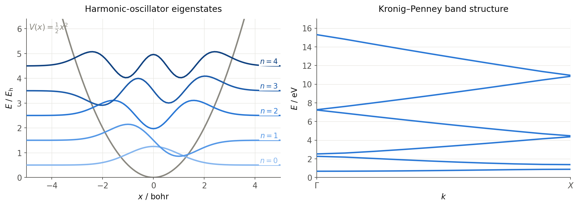
Harmonic-oscillator eigenstates and Kronig-Penney band structure computed with Numerov.jl

Left: the five lowest eigenstates of a 1D harmonic oscillator, computed from examples/1DHarmonicOscillator. Right: the band structure of a 1D Kronig-Penney model from examples/1DKronigPenney.

Installation

Requires Julia 1.10 or later. Numerov.jl is registered in the Julia General registry:

pkg> add Numerov

Quickstart

Numerov.jl has a single entry point: the exported function numerov reads an input file, solves the Schrödinger equation and writes all result files to the current working directory. On invalid input it throws a catchable ArgumentError rather than terminating Julia.

julia> using Numerov

julia> numerov("input.in")

or purely programmatically: solve_schrodinger takes the potential as an array and the grid axes as ranges, and returns the results as plain Julia values without touching any files —

julia> x = range(-5.0, 5.0; length = 201);

julia> solve_schrodinger(0.5 .* x .^ 2, x; n_eigenvalues = 3).energies
3-element Vector{Float64}:
 0.500000000049189
 1.5000000024036095
 2.5000000561274294

See library usage for 2D/3D problems, periodic systems, band structures and units.

The input file names a grid-potential file and sets calculation options — see the input file reference. Ready-to-run cases live in the examples/ directory of the repository, and a command-line interface is available as well.

Output files

All output files are written to the current working directory; existing files with the same names are overwritten on each run (eigenvalues.dat is deleted as soon as a run starts, since it is appended to per k-point).

File	Content	Written
`Numerov.out`	Log file: input parsing, system and sparse-matrix information (name configurable via `output-file`)	always
`eigenvalues.dat`	Eigenvalues in the chosen `potential-unit`, one line per k-point (k-point columns first for periodic runs)	always
`eigenvectors.dat`, `eigenvectors_shifted.dat`	Coordinates, potential and eigenvector amplitudes per grid point; the `shifted` variant offsets each eigenvector by its eigenvalue for plotting inside the potential	non-periodic runs
`eigenvectors_k_<k>.dat`, `eigenvectors_shifted_k_<k>.dat`, `imag_eigenvectors_k_<k>.dat`, `imag_eigenvectors_shifted_k_<k>.dat`	Real and imaginary parts of the (complex) eigenvectors, one set of files per k-point	periodic/k-point runs
`frequencies.dat` (or `frequencies_k_<k>.dat`)	Transition energies between the computed states as a lower triangular matrix, in `cm⁻¹`	always (per k-point for periodic runs)
`bandstructure.dat`	Distance along the k-path and the corresponding eigenvalues	only with `band-structure = on`
`timings.out`	Timing breakdown of the calculation (name configurable via `timings-file`)	always

Citing

If you use Numerov.jl in your research, please cite:

J. Gamper, F. Kluibenschedl, A. K. H. Weiss, T. S. Hofer, Accessing Position Space Wave Functions in Band Structure Calculations of Periodic Systems — A Generalized, Adapted Numerov Implementation for One-, Two-, and Three-Dimensional Quantum Problems, J. Phys. Chem. Lett. 2023, 14, 33, 7395–7403. doi:10.1021/acs.jpclett.3c01707

Citation metadata is also provided in CITATION.cff.