Analysis

All selected files form one ordered sequence in the browser. Mean, uncertainty, and histogram counts use all observations meeting the rules below. The MSER marker proposes an initial cut; it does not apply the cut.

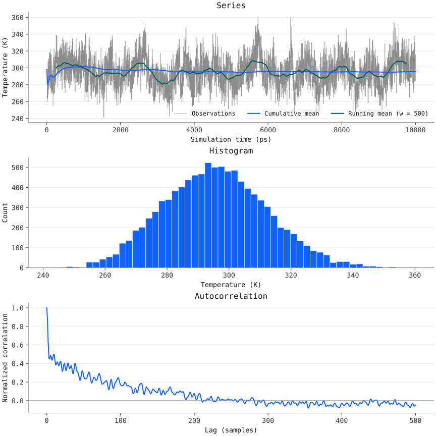
The same 10,000 observations in three views, from examples/md-01.en and examples/md-02.en. Reproduce this figure.

Charts and averages

View or guide	Definition	Interpretation
Series	Quantity against time or sample position	Range, changes, and outliers
Mean / median	Reference across all finite values	Location of the complete dataset
Cumulative average	Mean of finite observations up to each position	Sensitivity to accumulated history
Running average	Mean of a complete window of w samples, placed at its mean time	Local trend, not an uncertainty estimate
Histogram	Counts in shared bins over all finite values	Distribution of observations
Autocorrelation	The same mean-centered sequence against its lagged copy	Persistence of fluctuations in sample steps

The running window defaults to about 5% of the sequence, capped at 1,000 samples. The web interface clamps requested windows to the available data. Automatic histogram bins combine Sturges and Freedman–Diaconis rules, bounded for display. The optional Gaussian KDE is scaled to counts per bin; it is a smooth guide.

For long sequences, KDE fits a strided sample; histogram counts still use all finite observations.

Autocorrelation

For \(N\) finite values, let \(z_i=x_i-\bar{x}\). The estimate is

\[ r_k = \frac{\sum_{i=1}^{N-k} z_i z_{i+k}} {\sum_{i=1}^{N} z_i^2},\qquad r_0=1. \]

The denominator stays fixed at every lag; there is no \(N-k\) correction. Zero-padded FFT convolution avoids circular wrapping. The axis is lag in samples, even when the series uses physical time. Autocorrelation replaces the series while selected; it correlates the sequence with itself.

Uncertainty in the mean

The displayed ± value is an estimated standard error of the mean (SEM), not standard deviation or a confidence interval. The implementation uses population variance \(\sigma^2=N^{-1}\sum_i(x_i-\bar{x})^2\) and positive pairs \(r_1+r_2\), \(r_3+r_4\), …, stopping at the first nonpositive pair:

\[ g = \max\left(1,\ 1+2\sum_{k=1}^{2m}r_k\right),\qquad N_{\mathrm{eff}}=N/g,\qquad \mathrm{SEM}=\sigma\sqrt{g/N}. \]

Here \(m\) is the number of retained positive pairs. The interface reports τ = g in sample steps, using the full \(1+2\sum r_k\) convention. It does not use the alternative half-sized integrated-time convention. Positive-pair truncation is inspired by Geyer (1992), Practical Markov Chain Monte Carlo; the equations above specify this implementation’s pairing and normalization.

Interpret these estimates for a stationary sequence with regular sampling. Trends, irregular intervals, missing observations, or changed conditions require further review. Large \(N_{\mathrm{eff}}\) alone does not establish equilibration or adequate sampling of configuration space.

MSER cut

The batched MSER heuristic chooses a prefix length by minimizing the standard error of the remaining batch means. For \(N\) finite observations, batch size is \(\max(1,\lfloor N/\min(500,N)\rfloor)\). If this gives \(B\) complete batches, the retained tail has at least \(\max(2,\lfloor B/10\rfloor)\) batches. An incomplete final batch is excluded from this score. The earliest minimum wins. The cut index refers to the finite-value sequence.

This batched rule is based on White (1997), An Effective Truncation Heuristic for Bias Reduction in Simulation Output. It is not labelled MSER-5: batch size depends on sequence length. Review the proposed transient against physical observables and the simulation protocol before selecting data for a final estimate. Summary statistics continue to use the complete dataset.

Unavailable estimates

Condition	Behaviour
Nonfinite value	Gap in series; omitted from mean, histogram, SEM, and MSER
Window containing a nonfinite value	Running average unavailable for that window
Nonfinite value anywhere in the sequence	Autocorrelation unavailable; missing positions are not compressed
Fewer than two values or zero variance	Normalized autocorrelation unavailable
Fewer than four finite values, or arithmetic overflow	SEM and MSER unavailable
LOOPTIME, N(QM-ATOMS), N(SM-MOL), or any exactly constant series	Viewable diagnostic; no drift analysis or MSER marker

SEM and MSER omit nonfinite values, closing those gaps for calculation. Their sample-step correlation estimate therefore does not represent the original spacing when observations are missing. Cumulative averages retain missing positions as gaps and resume from the accumulated finite observations.

The summary’s standard deviation uses ddof=0. Drift, when available, is the second-half mean minus the first-half mean, divided by the overall standard deviation. It describes change; it is not a convergence test.