Getting started

Install

Use Python 3.12 or newer and a desktop browser with WebGL 2:

python3 -m venv .venv
source .venv/bin/activate
python -m pip install MolarVerse-PQViewer

Open a trajectory

pqviewer trajectory.xyz

Replace the path with your trajectory. PQViewer opens the default browser at http://127.0.0.1:8765. The Python package includes the interface; Node.js is needed only for frontend development.

The terminal shows the browser address and dataset size after startup. Press Ctrl+C to stop. --log-level defaults to info for data and analysis events; use debug for request logs, or warning / error for less output. pqviewer --help lists the options; pqviewer --version prints the installed version.

For the synthetic three-frame water example shown below:

curl -fsSLo water.xyz https://raw.githubusercontent.com/MolarVerse/PQViewer/main/examples/water.xyz
pqviewer water.xyz

With no path, pqviewer opens an empty workspace for Open or drag-and-drop. Use --no-open to open the browser yourself. For a server or compute node, follow Remote access, including institutional VPN and jump hosts.

Inspect and measure

1. Drag to rotate and scroll to zoom. Press R to fit the structure; C toggles the cell.

2. Click an atom to inspect its properties. Shift-drag a box to select a group.

3. For an ordered measurement, click the first atom. With Analyze open, press Shift+Tab to return to the canvas, then use ↑ / ↓ and Enter to add atoms in order. Two, three, or four atoms measure a distance, angle, or dihedral.

4. Use the timeline to change frames; Plot follows the measurement.

5. Use View for display settings and Export to save a figure.

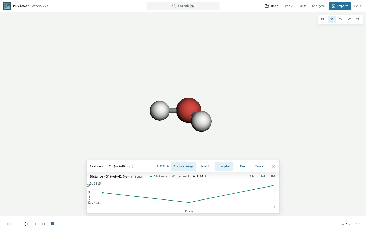
The synthetic water example above has its cell hidden. The plot shows minimum-image O–H distance in ångströms. See the viewer guide for selection, editing, and keyboard controls.

Other sources

Source	Command
PQ input	pqviewer simulation.in
One run or declared restart chain	pqviewer path/to/run-directory
Frames 100–999, every tenth frame	pqviewer 'trajectory.xyz@100:1000:10'

Slices use zero-based Python start:stop:step rules; the stop is exclusive. Quote a slice in the shell. Atom count and element order must stay stable; see source identity and periodic conventions.

Companion data

Unambiguous same-stem PQ companions are discovered automatically. Supply other paths explicitly:

pqviewer trajectory.xyz \
  --forces trajectory.force \
  --velocities trajectory.vel \
  --charges trajectory.chrg

Companion	Flags
Molecule, residue, and bond information	--moldescriptor moldescriptor.dat --topology topology
Scalar trajectory properties	--energy trajectory.en --info trajectory.info

--info requires --energy. Companion arrays must share the trajectory’s frame order and atom order; see alignment and units.

Optional workflows

Workflow	Install	Guide
ASE formats or Python Atoms	python -m pip install 'MolarVerse-PQViewer[ase]'	Data sources
Jupyter output cell	python -m pip install 'MolarVerse-PQViewer[jupyter]'	Jupyter
Headless figures	python -m pip install 'MolarVerse-PQViewer[render]', then python -m playwright install chromium	Figures and recipes

Release browser and rendering checks use Chromium on Linux. Other WebGL 2 browsers are outside that release coverage.