VACF and Spectra

The normalized velocity autocorrelation function describes how rapidly atomic velocities lose memory of their initial direction [Rahman1964], [Allen2017]:

\[C_{vv}(t) = \left\langle \frac{\sum_i \mathbf{v}_i(t_0)\cdot\mathbf{v}_i(t_0+t)} {\sum_i \mathbf{v}_i(t_0)\cdot\mathbf{v}_i(t_0)} \right\rangle_{t_0}.\]

The brackets denote an average over admissible time origins, and the sum runs over the selected atoms. This is the default, legacy-compatible estimator [thhTools] and gives \(C_{vv}(0)=1\). The fft estimator instead averages the numerator and denominator separately over all available origins before normalization, evaluating the correlation through the power spectrum as the Wiener-Khinchin theorem allows [Wiener1930], [Khintchine1934].

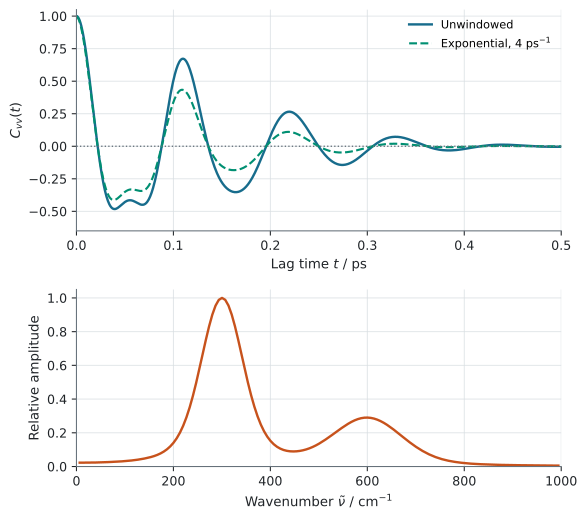
The cosine transform of the correlation is the vibrational density of states [Dickey1969], [Thomas2013]. If partial charges are supplied, PQAnalysis correlates \(q_i\mathbf{v}_i\) instead and the transform approximates an infrared spectrum [Thomas2013]. The analytic example below has two Gaussian-broadened bands at 300 and 600 cm⁻¹ with dephasing times of 0.22 and 0.12 ps; the dashed curve is the same correlation under an exponential window of 4 ps⁻¹, and both spectra are scaled to unit maximum.

Input

traj_files = trajectory.vel
target_selection = all
out_file = vacf.dat
time_step = 0.001
window = 2500
gap = 5
spectrum_file = spectrum.dat
ftsize = 5000
window_function = exponential
window_param = 4.0

Saved as vacf.in, it runs with:

$ pqanalysis vacf vacf.in

time_step is in ps. window is the maximum correlation lag in frames (the bundled Example data fixture uses window = 8); gap spaces the time origins. method = fft selects the denser-origin Wiener-Khinchin estimator.

The correlation written to out_file is never apodized. When a spectrum is requested, window_function (exponential, hann, blackman or the default none) multiplies a copy before the cosine transform [Harris1978]; the example applies \(\exp[-(4\ \mathrm{ps}^{-1})t]\). The optional windowed_out_file records that copy. The full key table is on VACFInputFileReader.

Output

out_file holds lag time and normalized correlation; spectrum_file holds wavenumber and relative amplitude (VACF and charge-flux correlation). In liquids, negative regions of the VACF indicate backscattering or cage motion; in solids, sign oscillations reflect bound vibrational motion. Charge-flux spectra are only as good as the partial charges behind them and are not absolute IR intensities. Discrete line spectra can be broadened separately with pqanalysis build_spectrum (Broadened spectrum).

Python

from PQAnalysis.analysis import VACF
from PQAnalysis.analysis.vacf import vacf_spectrum
from PQAnalysis.io import TrajectoryReader

time, correlation = VACF(
    TrajectoryReader("examples/water/trajectory.vel"),
    time_step=0.001,
    window_size=8,
    gap=2,
).run()
wavenumbers, amplitudes, windowed = vacf_spectrum(
    time,
    correlation,
    ftsize=5000,
    window_function="exponential",
    window_param=4.0,
)

vacf() runs an input file instead.

Before you trust it

• The Nyquist limit is set by the interval between written frames: 16678 cm⁻¹ at 1 fs, 1668 cm⁻¹ at 10 fs. Faster motion is aliased, not dropped.

• Resolution comes from window * time_step, about \(33.4 / T[\mathrm{ps}]\) cm⁻¹. ftsize only interpolates, and it truncates the correlation if it is smaller than window + 1.

• Apodization widens every band and lowers every peak; report the window and its parameter. hann and blackman do nothing until window_stop is set to the correlation length.

• Amplitudes are arbitrary units; the sum is not mass-weighted; peak positions are classical.

Each point is derived in VACF: Theory and Validity.