From trajectory to figure

This page runs one continuous Python session on examples/water: load the trajectory, inspect it, compute an RDF and an MSD, and plot.

Load and inspect

from PQAnalysis.io import read_trajectory

traj = read_trajectory("examples/water/trajectory.xyz")
frame = traj[0]
print(len(traj))                 # 25
print(frame.n_atoms)             # 3
print([atom.name for atom in frame.atoms])  # ['O', 'H', 'H']
print(frame.cell.box_lengths)    # [10. 10. 10.]

Check: 25 frames, three atoms, cubic 10 Å cell. If the atom count is wrong, stop; every later normalization will be wrong.

RDF of oxygen around hydrogen

from PQAnalysis.analysis import RDF
from PQAnalysis.io import TrajectoryReader

r, g, coordination, shell, residual = RDF(
    TrajectoryReader("examples/water/trajectory.xyz"),
    reference_species="O",
    target_species="H",
    delta_r=0.5,
    r_max=4.0,
).run()
print(r[0], g[0])                # 0.25  0.0
print(coordination[-1])          # 2.0  (both hydrogens)

Check: r_max = 4.0 is below half the shortest box edge (5 Å), so the minimum-image clamp is not in play. The first bin is empty (no O–H contact inside 0.5 Å); coordination saturates at 2.

MSD of the oxygen

from PQAnalysis.analysis import MSD

analysis = MSD(
    TrajectoryReader("examples/water/trajectory.xyz"),
    target_species="O",
    window=8,
    gap=2,
    time_step=0.001,
    fit_window=4,
)
lags, msd_x, msd_y, msd_z, msd_tot = analysis.run()
print(analysis.fit_results)

Check: one oxygen is selected. The Einstein fit uses the last four lag points of an eight-frame window; see MSD: Theory and Validity for choosing a real fit interval.

Plot

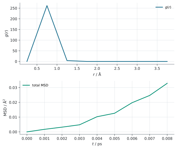
The arrays are plain NumPy arrays, so plotting is ordinary Matplotlib:

import matplotlib.pyplot as plt

fig, (ax_rdf, ax_msd) = plt.subplots(2, 1)
ax_rdf.plot(r, g)
ax_rdf.set(xlabel=r"$r$ / $\mathrm{\AA}$", ylabel=r"$g(r)$")
ax_msd.plot(lags * 0.001, msd_tot)
ax_msd.set(xlabel=r"$t$ / ps", ylabel=r"MSD / $\mathrm{\AA}^2$")
fig.tight_layout()
plt.show()

The same figure, with the documentation’s styling, is generated by the plot directive from docs/source/_plots/workflow.py:

To write the table instead of keeping arrays, use the file wrappers on Learn the Python API. Next: Atom selections and the method pages under Analyses.